The Hough Transform [Part 2]
Required Reading/Viewing:
Additional Reading
Recommended Jupyter Theme for presenting this notebook:
jt -t grade3 -cellw=90% -fs=20 -tfs=20 -ofs=20Last time we left off with two questions:

![]()
- To anwers these questions, we need to visit SRI (Stanford Research Institute) in the late 1960s.
- This was an interesting time at SRI. Researchers were building the world's first mobile robot, Shakey.

- One of the many problems SRI researchers faced in developing Shakey was creating a vision system that would allow Shakey to interpet the "Blocks World" he operated in.

- SRI Researchers Peter E. Hart and Richard O. Duda were looking for an efficient and reliable method for detecting lines in images.
- Hart + Duda likely used Robert's Cross or the Sobel-Feldman Operator to find edge pixels in images.
- They were then trying to use these images to "build a model of the local environment and to update the position of the robot from identificaion of known landmarks."

- In search for a solution, Peter Hart studied the first computer vision book (!), Azriel Rosenfeld's Picture Processing by Computer.
- In this book, Rosenfeld briefly mentions the then obscure Hough patent, describing the tranformation algabraically for the first time, and posed a simple and computationally efficient method of implementing Hough's method.

- However, Rosenfeld does not solve the intersection at $\infty$ problem.
- Simultaneously, Hart was examining another approach that he thought may be helpful in pattern recognition - integral geometry. This approach didn't work, but he did pick up a potentially useful alternative parameterization of a line.
- Let's have a look at this representation.

- Instead of parameterizing our line with a slope and y-intercept, here we're parameterizing our line using $\rho$ and $\theta$.
- $\rho$ is the distance from the origin to the closest point on our line
- $\theta$ is the angle between the positive side of our x-axis and a the chord connecting the origin to our line at a right angle
- Now that we've established this alternative line representation, we have an important little math puzzle to solve:
What is the equation of our line in terms of $\rho$ and $\theta$ ?
- Let's take this question one step at time.
- First, we need a strategy. One strategy is to use our familiar parameterization of a line $y = mx +b$, and try to figure out our slope $m$ and our y-intercept $b$ in terms of our new parameters $\rho$ and $\theta$.


![]()
![]()
Putting this all together, we have a new equation for a line in terms $\rho$ and $\theta$:
$$ y = -\frac{cos(\theta)}{sin(\theta)} x + \frac{\rho}{sin(\theta)} $$
We can re-arrange our new equation to make it a little more aesthetically pleasing:
$$ \rho = y sin(\theta) + x cos(\theta) $$
Let's make sure the form of our line makes sense:

![]()
Now, here's where it gets interesting. Hough used the common $y=mx+b$ representation of the line as the core of his transform, leading to an unbounded transform space. What Peter Hart saw here was a way to use this alternate representation of a line, $\rho = y sin(\theta) + x cos(\theta)$, to tranform our data into a more useful version of Hough's original space. Let's have a look at this transform!
from IPython.display import Image, display
from ipywidgets import interact

def slide_show(slide_num=0):
    '''Make a little slide show in the notebook'''
    display(Image('../graphics/hart_space/hart_space_' + str(slide_num) + '-01.png'))
interact(slide_show, slide_num = (0, 4));
- Using this alternate from of the line, our points are now transformed into pieces of sinusoids.
- As you may know, the sum of two sinusiods of the same variable is another sinusoid of the same variable.
- We can show this with little trigonometry or with Euler's formula.
- The really cool thing here is that, just as colinear points mapped to intersecting lines with Hough's tranform, co-linear points points map to intersecting curves in Hart's version of the transform.
- Now, remember that the real problem was that Hough's original space was unbounded - some co-linear points leds to lines that intersected at $\infty$.
- Let's see how our new space, introduced by Hart, handles this problem:
- As you can see, in our $\rho \theta$ space, we see intersections for both horizontal and vertical lines.
- In fact, we can represent $any$ line in $x, y$ space as a point in bounded $\rho, \theta$ space!
- So we've turned our problem of finding interecting points into a problem of finding interecting sinusoids. and made some real progress!
![]()
![]()
- Ok, one down one to go!
- Remember the whole idea here is to efficiently find noisy colinear points. This is what Hough set out to do for bubble chamber data, and what Hart and Duda needed to do to help shakey see make some sense of the world.
- The answer to this problem comes not from Duda, Hart, or Hough, but from Azriel Rosenfeld, the author of the very first computer vision book - Picture Processing by Computer.
def slide_show(slide_num=0):
    '''Make a little slide show in the notebook'''
    display(Image('../graphics/hough_accumulator/hough_accumulator_' + str(slide_num) + '.png'))
interact(slide_show, slide_num = (1, 3));
- Rosenfeld's solution began with quantizing the $\rho$, $\theta$ space into a grid
- Each cell in the grid represents an "accumulator"
- For each point in our image space $xy$, we map that point to a curve in $\rho \theta$ space, and increment the accumulator of each cell that our cuve pases through
- Rosenfeld's solution is quite powerful. By giving up some accuracy, we're able to efficiently compute an answer, and our quantization actualy makes our line detector less susceptable to noise!
- Quite often the Hough Transform is described as a "voting scheme", where each points votes for all the lines that could pass through it
From Wikipedia Hough Transform Article:
"The purpose of the technique is to find imperfect instances of objects within a certain class of shapes by a voting procedure. This voting procedure is carried out in a parameter space, from which object candidates are obtained as local maxima in a so-called accumulator space that is explicitly constructed by the algorithm for computing the Hough transform."
- Let's visualize this "voting" procedure one point at a time:

- Each point in our $xy$ space is mapped to sinusiodal curve in $\theta \rho$ space.
- For each cell of our accumulator that our curve passes through, we're incrementing our accumulator by one
- After we're done accumulating, the highest points in our accumulator space should correspond to the strongest lines in our image. Finding lines in our image should then just be a matter of finding the peaks in our hough space!
- Thanks to Hart and Duda, we now have a version of the Hough transform that is extremely useful for computer vision!
![]()
![]()
Implementation Time
Now that we understand the contributions of Hough, Rosenfeld, Hart, and Duda; it's time to implement their ideas in python. Let's think through the steps we need to implement.
- Transform the pixel indices of the points we would like to map into $xy$ coordinates
- Create an empty accumulator
- Map each point to a curve in parameter space using $\rho = y_i sin(\theta) + x_i cos(\theta)$, and for each cell that our curve passes through, increment our accumulator for the cell by one
- Identify lines in our original image using our accumulator values
It would probably be nice to have like, an image to work with. Let's import a brick image and use the Sobel-Feldman operator to compute/detect some potential edge pixels
%pylab inline
import os, sys
sys.path.append('..')

from util.filters import filter_2d
from util.image import convert_to_grayscale

im = imread('../data/easy/brick/brick_2.jpg')
gray = convert_to_grayscale(im/255.)
imshow(gray, cmap = 'gray');

#Implement Sobel kernels as numpy arrays
Kx = np.array([[1, 0, -1],
               [2, 0, -2],
               [1, 0, -1]])

Ky = np.array([[1, 2, 1],
               [0, 0, 0],
               [-1, -2, -1]])
Gx = filter_2d(gray, Kx)
Gy = filter_2d(gray, Ky)

#Compute Gradient Magnitude and Direction:
G_magnitude = np.sqrt(Gx**2+Gy**2)
G_direction = np.arctan2(Gy, Gx)
fig = figure(0, (6,6))
imshow(G_magnitude)

To detect thes edges, we only want to map strong edge pixels. Let's use a threshold to filter out non-edge pixels.
from ipywidgets import interact

#Show all pixels with values above threshold:
def tune_thresh(thresh = 0):
    fig = figure(0, (8,8))
    imshow(G_magnitude > thresh)
interact(tune_thresh, thresh = (0, 2.0, 0.05))
- A value of
thresh = 1.05looks pretty good to me! - Let's use this tresh to create and "edges" image:
edges = G_magnitude > 1.05
fig = figure(0, (6,6))
imshow(edges)

#How many points are we mapping?
sum(edges==1)
1. Transform the pixel indices of the points we would like to map into $xy$ coordinates
- We're now ready for our first step!
- edges is a 2-d numpy boolean array:
edges
We can find the indices of each "True" entry using the np.where method:
y_coords, x_coords = np.where(edges)
x_coords, y_coords
len(x_coords), len(y_coords)
As a check, let's scatter plot our coordinates:
fig = figure(0, (12,9))
scatter(x_coords, y_coords, s = 5)
grid(1)

Does anything look off about this plot to you?
![]()
![]()
fig = figure(0, (20,8))
fig.add_subplot(1,2,1)
imshow(edges)

fig.add_subplot(1,2,2)
scatter(x_coords, y_coords, s = 5)
grid(1)

Our image has been vertically flipped! Why?
- Our image has been flipped because of the way our coordinate systems are defined. Our image coorinate system's origin is the upper left corner of our image and positive is down, while our $xy$ coordinate system is defined in "the usual cartesian way".
- Technically we don't have to correct this - it's really just a matter of convention. However, making this correction will make things a little more consistent/easy-to-follow.
![]()
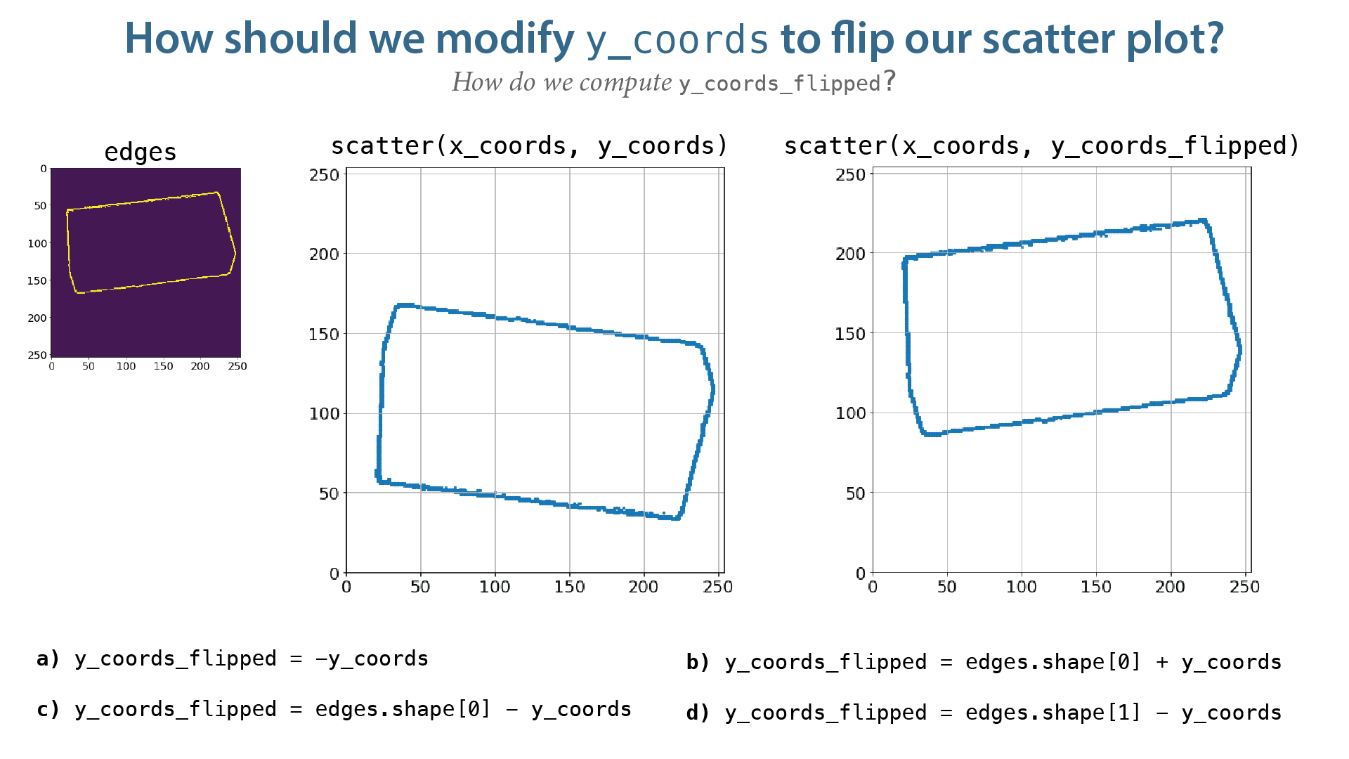
![]()
y_coords_flipped = edges.shape[0] - y_coords
fig = figure(0, (16,8))
ax = fig.add_subplot(1,2,1)
imshow(edges)

ax2 = fig.add_subplot(1,2,2)
scatter(x_coords, y_coords_flipped, s = 5)
grid(1)
xlim([0, edges.shape[0]]);
ylim([0, edges.shape[0]]);

Ok, now that our coordinates make some sense, we're ready for our next step.
2. Create an empty accumulator
We need to make some decision here about the size of our accumulator and the spacing of our accumulator grid cells. Let's start by picking the number of bins we want to use for $\rho$ and $\theta$.
#How many bins for each variable in parameter space?
phi_bins = 128
theta_bins = 128

accumulator = np.zeros((phi_bins, theta_bins))
So we have our accumulator, but there's one more important step here: we need to figure out what $\theta$ and $\rho$ values each cell in our accumulator actually correspond to. This depends on the range of phi and theta values we would like to cover. Fortunately, as we saw earlier, this set is bounded. However, it may not be immediately obvious what these bounds are. Let's explore this.

![]()
rho_min = -edges.shape[0]
rho_max = edges.shape[1]

theta_min = 0
theta_max = np.pi

#Compute the rho and theta values for the grids in our accumulator:
rhos = np.linspace(rho_min, rho_max, accumulator.shape[0])
thetas = np.linspace(theta_min, theta_max, accumulator.shape[1])
rhos
thetas
Alright, so we now have an empty accumulator, plus the $\rho \theta$ coordinates of each accumulator cell!
![]()
3. Map each point to a curve in parameter space using $\rho = y_i sin(\theta) + x_i cos(\theta)$, and for each cell that our curve passes through, increment our accumulator for the cell by one
So, we have these x_coords and y_coords_flipped that we need to map into parameter space.
len(x_coords)
x_coords
y_coords_flipped
scatter(x_coords, y_coords_flipped, s = 5)

- We'll interate through our points one at a time, and map them into paremeter space using our equation $\rho = y_i sin(\theta) + x_i cos(\theta)$.
for i in range(len(x_coords)):
    #Grab a single point
    x = x_coords[i]
    y = y_coords_flipped[i]

    #Actually do transform!
    curve_rhos = x*np.cos(thetas)+y*np.sin(thetas)

    for j in range(len(thetas)):
        #Make sure that the part of the curve falls within our accumulator
        if np.min(abs(curve_rhos[j]-rhos)) <= 1.0:
            #Find the cell our curve goes through:
            rho_index = argmin(abs(curve_rhos[j]-rhos))
            accumulator[rho_index, j] += 1
fig = figure(0, (8,8))
imshow(accumulator);

- Alright, we can make out some curves and some spikes in our parameter space!
- Let's have a look our accumulator in 3d.
#This is a complex plot - might run pretty slow!
from mpl_toolkits.mplot3d import Axes3D

fig = figure(figsize=(16, 16));
ax1 = fig.add_subplot(111, projection='3d')

_x = np.arange(accumulator.shape[0])
_y = np.arange(accumulator.shape[1])
_xx, _yy = np.meshgrid(_x, _y)
x, y = _xx.ravel(), _yy.ravel()

top = accumulator.ravel()
bottom = np.zeros_like(top)
width = depth = 1

ax1.bar3d(x, y, bottom, width, depth, top, shade = True);

4. Identify lines in our original image using our accumulator values
- In the accumulator plot above, which cells likely correspond to our lines in our original image?
![]()
- Large values in our accumulator should correspond to the intersection of lots of curves in our parameter space, which should correpond to strong lines in our original image.
- So what we're looking here for is large values or spikes in our accumulator space.
- There are lots of numerical methods for finding peaks in n-dimensional data, but let's start with something simple.
- Let's start by finding the max acccumulator value.
max_value = np.max(accumulator)
max_value
Now, let's find all the accumulator values above some percentage of our maximum.
def tune_thresh(relative_thresh = 0.9):
    fig = figure(0, (8,8))
    imshow(accumulator > relative_thresh * max_value)
interact(tune_thresh, relative_thresh = (0, 1, 0.05))
Let's threshold our accumulator:
relative_thresh = 0.35

#Indices of maximum theta and rho values
rho_max_indices, theta_max_indices,  = np.where(accumulator > relative_thresh * max_value)
theta_max_indices, rho_max_indices
Now, let's find the values of $\rho$ and $\theta$ that correspond to these indices. We can do this by sampling our arrays from earlier:
thetas_max = thetas[theta_max_indices]
rhos_max = rhos[rho_max_indices]
thetas_max, rhos_max
Ok, we can now plot the lines that correspond to these $\theta$, $rho$ values in our original image! We'll use our rearrangement of our line equation from ealier, $y = -\frac{cos(\theta)}{sin(\theta)} x + \frac{\rho} {sin(\theta)}$.
fig = figure(0, (8,8))
imshow(im)

for theta, rho in zip(thetas_max, rhos_max):
    #x-values to use in plotting:
    xs = np.arange(im.shape[1])

    #Check if theta == 0, this would be a vertical line
    if theta != 0:
        ys = -cos(theta)/sin(theta)*xs + rho/sin(theta)

    #Special handling for plotting vertical line:
    else:
        xs = rho*np.ones(len(xs))
        ys = np.arange(im.shape[0])

    #have to re-flip y-values to reverse the flip we applied initially:
    plot(xs, im.shape[0]-ys)

xlim([0, im.shape[0]]);
ylim([im.shape[1], 0]);

We Win!
- That's to Hough's Idea, Rosenfeld's suggestions, and Hart + Duda final touches, we've been able to detect lines in our images!
- Now, our detection isn't perfect, and there's lots of parameters for us to tune + play with, but we've got the core idea here of one of the most prolific algorithms in computer vision! Searching "Hough Transform" on Google Scholar returns 121,000 matches!

Final word from Peter Hart on the Hough Transform
I reached out to Peter Hart and asked how important his modified Hough Transoform was to the Shakey project, he responded (!) and had this to say:
"To answer your question, our modified transform was probably the most important tool we had in our computer vision toolbox. I don’t know if you’ve run across the 5 minute video that SRI made for the IEEE event celebrating the recognition of Shakey as a Milestone in the history of electrical engineering and computing. If you look at around 2:30 mark for a few seconds you’ll see the processing steps that extracted a room’s baseboards from an image. We used the transform to fit lines to the points, from which we could pinpoint the location of the corner of the room. That information was used to update Shakey’s position— the position being approximated by dead reckoning based on counting pulses in the stepping motors that drove Shakey, a process that accumulates errors.
A similar process was used to find the bases of the big geometric objects, which is also at least hinted at in the short video.
This transform-based image analysis was so effective that we never seriously used our home-made, triangulating laser range finder, that you’ve probably noticed in images of Shakey. We had thought we’d need it at the least for determining the distance to walls, since we knew the dead reckoning system needed periodic position updates. But vision alone did the trick.
I don’t know if you’ve come across these specs, but our vidicon-tube based imaging system, complete with home-made A-D converter (no such thing as a frame grabber then), delivered an image that was 120 x 120 pixels 4 bits deep. Try to get your head around those numbers next time you glance at the specs on your phone’s camera."
- Personal Correspondance with Peter Hart
- You can imagine how the Hough Transform may be helpful in the challenge for this module!
- Interestingly, the Hough Transform can be modified to work with other shapes, such as circles.
- We'll cover this if we have time, if not it may be worth looking into yourself, as it could be quite helpful on the coding challenge.
Appendix A - Wrapped up Hough Accumulator
class HoughAccumulator(object):
    def __init__(self, theta_bins, phi_bins, phi_min, phi_max):
        '''
        Simple class to implement an accumalator for the hough transform.
        Args:
        theta_bins = number of bins to use for theta
        phi_bins = number of bins to use for phi
        phi_max = maximum phi value to accumulate
        phi_min = minimu phi value to acumulate
        '''
        self.accumulator = np.zeros((phi_bins, theta_bins))

        #This covers all possible lines:
        theta_min = 0
        theta_max = np.pi

        #Compute the phi and theta values for the grids in our accumulator:
        self.rhos = np.linspace(rho_min, rho_max, self.accumulator.shape[0])
        self.thetas = np.linspace(theta_min, theta_max, self.accumulator.shape[1])

    def accumulate(self, x_coords, y_coords):
        '''
        Iterate through x and y coordinates, accumulate in hough space, and return.
        Args:
        x_coords = x-coordinates of points to transform
        y_coords = y-coordinats of poits to transform

        Returns:
        accumulator = numpy array of accumulated values.
        '''

        for i in range(len(x_coords)):
            #Grab a single point
            x = x_coords[i]
            y = y_coords[i]

            #Actually do transform!
            curve_prho = x*np.cos(self.thetas)+y*np.sin(self.thetas)

            for j in range(len(self.thetas)):
                #Make sure that the part of the curve falls within our accumulator
                if np.min(abs(curve_rhos[j]-self.rhos)) <= 1.0:
                    #Find the cell our curve goes through:
                    rho_index = argmin(abs(curve_rhos[j]-self.rhos))
                    accumulator[rho_index, j]+=1

        return accumulator

    def clear_accumulator(self):
        '''
        Zero out accumulator
        '''
        self.accumulator = np.zeros((phi_bins, theta_bins))
Appendix B - Downloading Data + Videos
#(Optional) Download data + videos if you don't have them.
import os, sys
sys.path.append('..')
from util.get_and_unpack import get_and_unpack

if not os.path.isdir('../data/'):
    url = 'http://www.welchlabs.io/unccv/the_original_problem/data/data.zip'
    get_and_unpack(url, location='..')

if not os.path.isdir('../videos/'):
    url = 'http://www.welchlabs.io/unccv/the_original_problem/videos.zip'
    get_and_unpack(url, location='..')